A satellite orbiting at 705 kilometers cannot stick a probe into your soil. What it can do is measure how your soil reflects specific wavelengths of electromagnetic radiation — and those reflectance patterns carry more information about soil organic carbon than most agronomists initially expect. Understanding both the physics and the limitations is essential before relying on spectral data in an MRV context.
The Physics of Soil Reflectance
When sunlight strikes bare soil, different soil constituents absorb and scatter radiation differently across the electromagnetic spectrum. In the visible range (400–700 nm), organic matter and iron oxides are dominant absorbers — both darken the soil. In the near-infrared (NIR, 700–1,000 nm), the soil matrix, clay minerals, and soil moisture interact with radiation in ways that carry structural information. In the shortwave infrared (SWIR, 1,000–2,500 nm), two especially informative regions emerge.
The SWIR1 region (approximately 1,550–1,750 nm, corresponding to Sentinel-2 Band 11 at 20-meter resolution) shows consistent inverse correlation with soil organic carbon content in mineral agricultural soils. The mechanism involves the absorption features of organic compounds — specifically O-H and C-H stretch overtones — that become more pronounced as organic carbon concentration increases. The SWIR2 region (approximately 2,090–2,350 nm, Sentinel-2 Band 12) carries complementary information, particularly useful for distinguishing organic carbon from clay mineral effects, since aluminosilicate clay minerals have characteristic absorption features in this band.
The practical result: a bare soil pixel with 3.5% SOC reflects less SWIR1 and SWIR2 radiation than a pixel with 1.5% SOC, all else being equal. That difference is measurable from space with current satellite hardware.
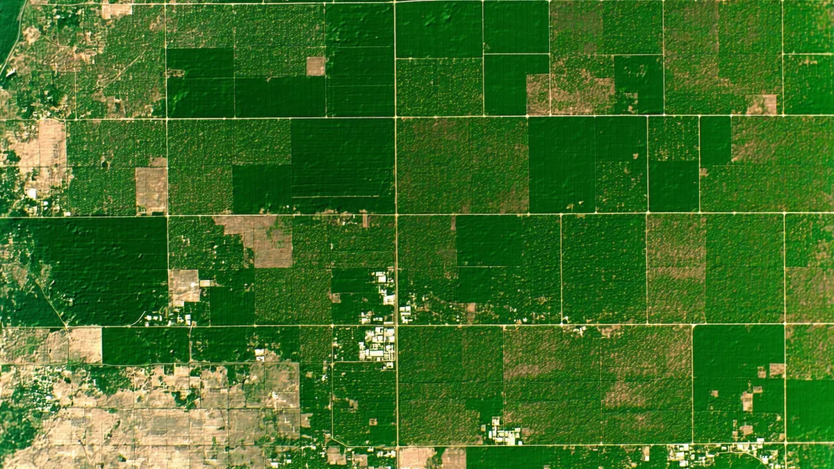
Sentinel-2 and Landsat 9: What the Platforms Actually Provide
Sentinel-2 (ESA, Copernicus program) offers 20-meter spatial resolution in its SWIR bands with a 5-day revisit cycle for a given location when both Sentinel-2A and 2B are operational. This temporal density is critical for MRV: it allows acquisition of cloud-free bare-soil composites by stacking multiple passes and selecting scenes with minimal vegetation cover or cloud contamination.
Landsat 9 (USGS/NASA) provides 30-meter spatial resolution in its SWIR bands (Bands 6 and 7, equivalent in spectral range to Sentinel-2 Bands 11 and 12), with a 16-day revisit. Landsat's value lies partly in its archive — continuous imagery since 1972 means historical bare-soil composites can be constructed for baseline context, though for regulatory-grade baseline measurements, physical samples remain necessary.
For operational MRV, both platforms are used in complementary fashion. Sentinel-2's higher spatial resolution and more frequent revisit provide the primary time-series; Landsat 9 adds depth to multitemporal compositing. Both are freely available through ESA's Copernicus Open Access Hub and USGS EarthExplorer — not proprietary commercial sensors, which is an important point for protocol compliance and independent auditability.
The Confounding Factors (This Is Where It Gets Complicated)
Soil spectroscopy from space would be a complete solution if soil reflectance only varied with SOC. It doesn't.
Soil moisture is the dominant confounding factor. Wet soil reflects less SWIR radiation than dry soil, regardless of organic carbon content. A rainfall event two days before a satellite pass can produce spectral values that look like a significant SOC increase. This is why bare-soil compositing — selecting only scenes acquired under low soil moisture conditions — is an essential pre-processing step. It's operationally feasible in the Midwest, where extended dry periods after harvest allow good bare-soil composites in autumn, but it constrains the effective monitoring window.
Clay mineralogy creates location-specific interference in SWIR2. High-clay soils (particularly those with significant smectite or kaolinite content) show spectral features that overlap with SOC absorption. Iowa Mollisols, which dominate the enrolled farm areas Terrabit works with, are generally well-characterized in terms of clay composition through USDA NRCS soil survey data, enabling model correction. But applying a model calibrated on Iowa Mollisols to a soil series in a different region without recalibration would produce unreliable estimates.
Surface roughness and tillage artifacts affect directional reflectance. A freshly tilled field with large clod structure scatters light differently than a smooth, compacted surface — a purely physical effect that the spectral signal can't distinguish from organic matter changes without ancillary data about field operations.
Crop residue is perhaps the most operationally challenging factor for regenerative agriculture specifically. No-till and cover crop systems — the exact management practices that build SOC — also leave more crop residue on the soil surface. Residue has distinct spectral features, particularly the cellulose absorption feature at approximately 2,100 nm, that must be spectrally unmixed from the soil signal. Several residue index approaches exist in the literature (Crop Residue Index, Shortwave Angle Slope Index), but this remains an active area of methodological refinement.
We're not saying satellite spectroscopy alone can verify a carbon credit. We're saying it's a powerful continuous monitoring tool that, properly calibrated against physical ground truth, dramatically expands what's observable between sampling campaigns.
How Calibration Against Ground Truth Works
The operational procedure begins with a soil core sampling campaign timed to coincide with a bare-soil satellite acquisition window — typically late October through early December in central Iowa, after harvest and before freeze. Soil cores are collected at a density appropriate for the farm's spatial heterogeneity (typically 1 core per 10–20 acres for initial calibration), processed for SOC via loss-on-ignition or dry combustion (Dumas method), and lab-analyzed to produce a set of known-SOC points with precise geographic coordinates.
Those points are then matched to the corresponding satellite pixels in the temporal composite — bare-soil reflectance values in SWIR1 and SWIR2 at each sample location. The empirical relationship between reflectance and measured SOC is modeled using regression approaches ranging from simple linear models to partial least squares regression (PLSR) or machine learning regressors depending on sample density and spectral complexity. The farm-specific model is then applied to the full spatial extent of the field to estimate SOC at all pixels, with uncertainty quantified via cross-validation.
Consider how this played out in practice at a 1,800-acre operation in Mahaska County, Iowa in the autumn of 2023. The farm had been practicing no-till corn-soybean rotation for six years. We collected 94 soil cores stratified by soil mapping unit, targeting a coefficient of variation below 15% in the predicted SOC estimates. The PLSR model calibrated on these samples achieved a root mean square error of prediction (RMSEP) of 0.18% SOC in cross-validation — tight enough to detect the 0.3–0.6% SOC increases expected over a typical 3-year regenerative management period.
Temporal Change Detection
The most important application of satellite spectroscopy in the MRV context isn't the single-point SOC estimate — it's the temporal change signal. Annual bare-soil composites from the same field, processed consistently, provide a time series in which trends in spectral reflectance can be interpreted as trends in SOC, subject to the calibration and confounding factor corrections described above.
This temporal record serves two functions. First, it provides continuous monitoring between physical sampling campaigns, flagging fields where spectral trends diverge from expectations (which may indicate management changes, soil disturbance, or data collection errors requiring investigation). Second, it provides spatial interpolation across the farm — physical cores anchor absolute SOC values at sampled points, while the satellite time series propagates those values to unsampled areas with documented uncertainty.
The combination allows a sampling density — and therefore a measurement cost — that would be economically impossible with physical cores alone, while maintaining the accuracy constraints required for protocol-grade MRV. It's not a shortcut; it's a spatial scaling methodology with quantified confidence bounds. The difference matters for how the output is interpreted and how the uncertainty is disclosed in a credit package.
What Satellite Spectroscopy Cannot Do
Spectral reflectance is a surface measurement. Sentinel-2 and Landsat 9 are sensing the top few millimeters of soil at best — the optical depth of SWIR reflectance in agricultural soils is typically less than 1 mm. SOC at depth (30–60 cm, 60–90 cm) is invisible to these sensors. Subsoil carbon accumulation, which can be significant under perennial cover crops and deep-rooted species, requires physical sampling — there's no remote sensing workaround for deep horizon measurements.
Similarly, spectral data cannot establish a legal baseline for credit issuance without physical corroboration. Registry protocols require direct measurement at baseline; satellite data cannot substitute for that initial physical campaign. What satellite data provides is cost-effective continuous monitoring between sampling events and spatial interpolation within enrolled fields. The protocol requires both, and Terrabit's methodology is designed so that neither is treated as optional.
Written by the Terrabit Science Team. For methodology questions or to discuss spectral calibration for your operation, contact [email protected].